Lost Jobs in Recessions

The WSJ has a nice article showing just how hard it has been for many people who lost jobs in the recession to get back to work. Their profile is typical of what I have read and not the typical picture of unemployment: Middle age middle managers. The paper by Steve Davis and Till von Wachter is here. They present the fact largely as a puzzle, which it is:  "losses in the model vary little with aggregate conditions at the time of displacement, unlike the pattern in the data."

As the story makes clear, the problem is really not unemployment. There are lots of jobs available. The jobs just don't pay much, and don't use the specialized skills that the workers have to offer. The problem is wages at the jobs they can get.

This is a very interesting fact, with many less than obvious interpretations. It strikes me as a good teaching moment for economics classes.

The natural interpretation of all correlations is causal: There are  two identical workers in two identical jobs at two identical companies. One worker happened to lose his or her job in a recession, and so faces a harder climb back. We learn about the difference in job markets over time.

Maybe, but the job of being an economist is to recognize lots of other possibilities for a correlation. So the proposed discussion question: what else might this mean? How does taking averages reflect selection rather than cause?

Perhaps not all workers are the same. The conventional view of recessions is that companies fire people from lack of "aggregate demand," or shocks external to the firm.  In good times, companies fire people when those people aren't very good. Then, you would think, being laid off in a recession is better than being laid off in good times. If you're laid off in good times that is a signal you're not a great worker. In a recession, everybody got laid off, so there is not any particular stigma in it.  Well, so much for that story.

A contrary story is that it's easier to get rid of people in a recession. The head of a large business once told me how useful the last recession was, as he could plead financial problems and finally get rid of the army of unionized workers that were playing solitaire all day. Guido Menzio  and Mikhail Golosov have a model that (I think!) formalizes this story. (Menzio was recently in the news, as an idiot fellow passenger thought he was a terrorist because he was doing algebra on a plane, a different sad commentary on contemporary America.)

Perhaps not all businesses are the same. Businesses and occupations that get hit in recessions are different from those that get hit in booms...

Perhaps times are not the same. Recessions are pretty much by definition a time when different sorts of shocks hit the economy. If recession shocks require bigger changes in specialized human capital than normal-times (more idosyncratic shocks), or people to move industries and cities more, then you'll see this pattern.

And so on. Interesting facts, not so obvious interpretations, averages that don't always mean what you think they mean, that's why economics is so fun.

Update:  Steve Davis writes to explain that job losses in recessions are concentrated in specific industries:

You write: "...If recession shocks require bigger changes in specialized human capital than normal-times (more idiosyncratic shocks), or people to move industries and cities more, then you'll see this pattern.” 

Here’s a modified version of this story that has more promise in my view.  First, an under appreciated empirical observation: The cross-industry (cross-firm, cross-establishment) distribution of employment growth rates becomes more negatively skewed in recessionary periods.  Job loss is also concentrated in industries (firms, establishments) that experience relatively large net and gross job destruction rates.  Taken together, these two observations tell us that, in recessions, a larger share of job losers hail from industries (firms, establishments) that get hit by especially large negative shocks (even compared to the average), reducing the value of skills utilized by workers in those industries (firms, establishments).  I conjecture that negative skewness in the cross-occupation distribution of employment growth rates is also counter cyclical, but I don’t recall any direct and convincing evidence on that score. 

Restating, the setting in which job loss occurs worsens for the average job loser in recessions, because (1) overall economic conditions worsen in recessions, AND (2) conditions worsen especially for industries (occupations, etc.) with a disproportionate share of job loss. Many models consider the effects of (1), but there is little work on (2).  Testing hypotheses and building theories related to (2) requires good measures of the individual-specific “setting” in which individual job losses occur.  One of my PhD students, Claudia Macaluso, is making good progress on that front in her dissertation.

William Carrington and Bruce Fallick have a review paper on why earnings fall with job displacement.

Global Imbalances

I gave some comments on “Global Imbalances and Currency Wars at the ZLB,” by Ricardo J. Caballero, Emmanuel Farhi, and Pierre-Olivier Gourinchas at the conference, “International Monetary Stability: Past, Present and Future”, Hoover Institution, May 5 2016. My comments are here, the paper is here 

The paper is a very clever and detailed model of "Global Imbalances," "Safe asset shortages" and the zero bound. A country's inability to "produce safe assets" spills, at the zero bound, across to output fluctuations around the world. I disagree with just about everything, and outline an alternative world view.

A quick overview:

Why are interest rates so low? Pierre-Olivier & Co.: countries can't  “produce safe stores of value”
This is entirely a financial friction. Real investment opportunities are unchanged. Economies can’t “produce” enough pieces of paper. Me: Productivity is low, so marginal product of capital is low.

Why is growth so low? Pierre-Olivier: The Zero Lower Bound is a "tipping point." Above the ZLB, things are fine. Below ZLB, the extra saving from above drives output gaps. It's all gaps, demand. Me: Productivity is low, interest rates are low, so output and output growth are low.

Data: I Don't see a big change in dynamics at and before the ZLB. If anything, things are more stable now that central banks are stuck at zero. Too slow, but stable.  Gaps and unemployment are down. It's not "demand" anymore.


Exchange rates. Pierre-Olivier  "indeterminacy when at the ZLB” induces extra volatility. Central banks can try to "coordinate expectations." Me: FTPL gives determinacy, but volatility in exchange rates. There is no big difference at the ZLB.

Safe asset Shortages. Pierre-Olivier: driven by a large mass of infinitely risk averse agents. Risk premia are therefore just as high as in the crisis. Me: Risk premia seem low. And doesn't everyone complain about "reach for yield" and low risk premia?

Observation. These ingredients are plausible about fall 2008. But that's nearly 8 years ago! At some point we have to get past financial crisis theory to not-enough-growth theory.

But, finally, praise. This is a great paper. It clearly articulates a world view, and you can look at the assumptions and mechanisms and decide if you think they make sense. I am in awe that Pierre-Olivier & Co. were able to make a coherent model of these buzzwords.

But great theory is great theory. To a critic, the assumptions are necessary as well as sufficient. I  read it as a brilliant negative paper, almost a parody: Here are the extreme assumptions that it takes to justify all the policy blather about "savings gluts" "global imbalances" "safe asset shortages" and so on. To me, it shows just how empty the idea is, that our policy-makers understand any of this stuff at a scientific, empirically-tested level, and should take strong actions to offset the supposed problems these buzzwords allude to.

I hope this taste gets you to read  my comments and the paper. 

Delong and Logarithms

Brad Delong posted a response to my oped on growth  in the Wall Street Journal. He took issue with my graph, reproduced here,

by making his own graph, here

He characterizes the difference between our graphs with his usual gentlemanly restraint,

"Extraordinarily Unprofessional!!:" "total idiocy" The University of Chicago and the Wall Street Journal Have Very Serious Intellectual Quality Control Problems

and so forth.

If you read Brad, you may wonder what skulduggery I used to make the plot. I will now reveal the dark secret. It's a clever Chicago-school mathematical trick:

Logarithms.

Yes, I plotted log income vs. ease of doing business index.

Now just how much of a sin is this? Well, growth theory is about growth, so it's pretty hard to do without logarithms. If thinking about percentage growth and running regressions with log income on the left hand side is a devious right-wing trick, I'm afraid we're going to have to throw out about 99% of growth theory and empirical economics, including much done by Brad's colleagues at Berkeley.

Furthermore, just look at the graph.  I invite anybody who has sat through a first-year econometrics class where they teach this devious technique to ponder my and Brad's plot, and think whether a level or a log fit is appropriate.

Brad raises one valid concern with all of empirical economics: Endogeneity. The graph is a correlation. How do we know that better ease of doing business causes better business, and not the other way around? In Brad's view, it is equally likely, I guess, that first a contry gets rich, and then it improves its laws and regulations.

I didn't mention this in the Journal, simply for lack of space (try to write anything in 950 words). In a previous blog post, here, I wrote a little bit about it.

One might dismiss the correlation a bit as reverse causation. But look at North vs. South Korea, East vs. West Germany, and the rise of China and India. It seems bad policies really can do a lot of damage. And the US and UK had pretty good institutions when their GDPs were much lower. (Hall and Jones 1999 control for endogeneity in this sort of regression by using instrumental variables.)

(This post isn't hard to find. I linked to from my growth oped post. And if one is curious about "what does John have to say about endogeneity?" -- a rather obvious question, which I ask about twice at every seminar -- it is also possible to email me. )

That post goes on to survey a lot of academic literature on just how important good institutions are to economic growth.

But just think about it. Did North Korea or East Germany first get poor and then get bad institutions? Did the UK and US first get rich, and then develop our rule-of-law and property rights traditions? Is reverse causality at all a plausible explanation for the correlation? Just about every historical episode you can think of goes the other way.

Endogeneity is always an issue in economics, but Brad's case that I am too dumb to have even thought about it, or that this correlation obviously goes the other way,  does not hold up.

But apparently, Brad doesn't know about google, fact checking, or emailing for simple clarifications either. Otherwise he would know that I don't work at Chicago anymore, hardly a secret.

The notion that universities should practice "intellectual quality control" is interesting in this era of declining free speech. Brad, be careful what you wish for.  "Controlling" basic professional ethics may come first.

If anyone is still curious, I posted my data and program to my website, and this post describes it some more. I didn't clean it up well, as I never thought this would be controversial, but at least it documents what I did. Feel free to play with it as you wish.

Update: It's clear from many comments and the twitter storm that many readers, even trained economists, missed this basic point. My graph is an illustration of a conclusion reached by hundreds, if not more, papers in the academic literature. It is not The Evidence, or even particularly novel evidence. Were it so, standard errors, specification search, endogeneity, much better measures of institutions, etc. would be appropriate, as many suggest. My graph is just a quick graphical illustration of the conclusions of much growth economics, including much work by Jones, Acemoglu, Barro, Klenow, and many many others. Institutions matter to economic growth; bad governments have amazing power to ruin economies.  As always in writing, I should have made that clearer; but I thought this literature was familiar to the average economist-blogger.

Update 2: There is, I think, an important mis-specification in a regression of log income on the ease-of-doing business index, which Evan Soltas implicitly points out.  I referred to the index as "simple" and "crude" for this reason, but again it looks like this seemingly obvious point needs expanding.

The World bank's measure is mostly focused on the ease of starting small businesses. When we look at the regulatory sclerosis in the US, it is a much wider phenomenon, encompassing the tax code, social program disincentives, the  recent huge expansion of federal involvement in health and finance, general spread of cronyism, reduction in rule of law, and so forth. These affect large businesses as much or more than small businesses.

Clearly, as we look across countries, the ease of doing business is correlated with these wider legal and regulatory problems. Countries with bad institutions overall also have bad ease of doing business scores. But just as obviously, only fixing the ease of doing business indicators without fixing the larger legal and institutional failures that correlate with those indicators, won't do a whole lot of good, which is what Evan seems to find.

The regulatory program I outlined there and in the longer essay on growth (blog post here, html here,   pdf here) went far beyond ease of doing business indicators, for just this reason.

Update 3: Or, seemingly obvious point #3 that seems to need an answer. A few commenters have questioned  how far "out of sample" one can go. At some point, yes, institutions are perfect and more income will not result from improving them. Where is that? 90? 100? 110? I don't know. But the local derivative is still high, no matter how you fit the "out of sample" points. If you don't think you can draw the line out to 100, going from 82 to 83 still has very large effects.

Central Bank Governance and Oversight Reform

The Hoover Institution Press just published "Central Bank Governance and Oversight Reform," the collected volume of papers, comments, and discussion from last May's conference here by the same name. You can get the  book or e-book here at the Hoover press or here at amazon.com. The individual chapter pdfs are available here.  Press release here.

(My modest contributions are in the preface and a discussion of Paul Tucker's Chapter 1. I agree it would be nice to have a more rule-based approach to lender of last resort and bailout functions, but wouldn't lots of equity so you don't have to mop up so often be even better?)

This is part of an emerging series of monetary policy conferences at Hoover. Tomorrow we will have a conference on international monetary policy. Stay tuned...

The blurb:

How can we balance the central bank’s authority, including independence, with accountability and constraints? Drawn from a 2015 Hoover Institution conference, this book features distinguished scholars and policy makers’ discussing this and other key questions about the Fed. Going beyond the simple decision of whether to raise interest rates, they focus on a deeper set of questions, including, among others, How should the Fed make decisions? How should the Fed govern its internal decision-making processes? What is the trade-off between greater Fed power and less Fed independence? And how should Congress, from which the Fed ultimately receives its authority, oversee the Fed?

The contributors discuss, for instance, whether central banks can both follow rule-based policy in normal times but then take a discretionary, do-what-it-takes approach to stopping financial crises. They evaluate legislation, recently proposed in the U.S. House and Senate, that would require the Fed to describe its monetary policy rule and, if and when the Fed changed or deviated from its rule, explain the reasons. And they discuss to best ways to structure a committee—like the Federal Open Market Committee, which sets interest rates—to make good decisions, as well as offer historical reflections on the governance of the Fed and much more. They conclude with an important reminder: how important it is to have a “healthy separation between government officials who are in charge of spending and those who are in charge of printing money,” the most essential part of good governance.

The contents:

Preface
By John H. Cochrane and John B. Taylor

Chapter 1: How Can Central Banks Deliver Credible Commitment and Be “Emergency Institutions”?
By Paul Tucker

Chapter 2: Policy Rule Legislation in Practice
By David H. Papell, Alex Nikolsko-Rzhevskyy and Ruxandra Prodan

Chapter 3: Goals versus Rules as Central Bank Performance Measures
By Carl E. Walsh

Chapter 4: Institutional Design: Deliberations, Decisions, and Committee Dynamics
By Kevin M. Warsh

Chapter 5: Some Historical Reflections on the Governance of the Federal Reserve
By Michael D. Bordo

Chapter 6: Panel on Independence, Accountability, and Transparency in Central Bank Governance
By Charles I. Plosser, George P. Shultz, and John C. Williams

Macro Musing Podcast

I did a podcast with David Beckworth, in his "macro musings" series, on the Fiscal Theory of the Price Level, blogging, and a few other things.



(you should see the link above, if not click here to return to the original).

You can also get the podcast at Sound Cloud, along with all the other ones he has done so far, or on itunes here.  For more information, see David's post on the podcast.

Blinder on Trade

Alan Blinder has an excellent op-ed in the WSJ on trade. It's hard to excerpt as every bit is good.

1. Most job losses are not due to international trade. Every month roughly five million new jobs are created in the U.S. and almost that many are destroyed, leaving a small net increment. International trade accounts for only a minor share of that staggering job churn. ...

2. Trade is more about efficiency—and hence wages—than about the number of jobs. You probably don’t sew your own clothes or grow your own food. Instead, you buy these things from others, using the wages you earn doing something you do better.  ...

3. Bilateral trade imbalances are inevitable and mostly uninteresting. Each month I run a trade deficit with Public Service Electric & Gas. They sell me gas and electricity; I sell them nothing....

4. Running an overall trade deficit does not make us “losers.”...

5. Trade agreements barely affect a nation’s trade balance. ..a nation’s overall trade balance is determined by its domestic decisions, not by trade deals... America’s chronic trade deficits stem from the dollar’s international role and from Americans’ decisions not to save much, not from trade deals. Trade deficits are not a major cause of either job losses or job gains. ...trade makes American workers more productive and, presumably, better paid.

One could say much more. Trade is not a "competition," for example. But,  having done this sort of thing, I'm sure lots of other good bits are on the cutting room floor.

Alan is more sympathetic to government "help" to trade losers, which I agree sounds nice if it were run by the benevolent and omniscient transfer payment planner, but I think works out poorly in practice when we look at the success or failure of actual trade adjustment programs. But that is a small nitpick.

Alan closes by wishing that Bernie Sanders and Donald Trump understood these simple facts a bit better. I think his list of politicians needing enlightenment could be a little longer. But he's courageous enough for speaking the kind of heretical truth that will come back to haunt him should he ever want a government job.

Chari and Kehoe on Bailouts

V. V. Chari and Pat Kehoe have a very nice article on bank reform, "A Proposal to Eliminate the Distortions Caused by Bailouts," backed up by a serious academic paper.

Their bottom line proposal is a limit on debt to equity ratios, rising with size. This is, I think, a close cousin to my view that a Pigouvian tax on debt could substitute for much of our regulation.

Banks pose a classic moral hazard problem. In a financial crisis, governments are tempted to bail out bank creditors. Knowing they will do so, bankers take too much risk and people lend to too risky banks. The riskier the bank, the stronger the governments' temptation to bail it out ex-post.

Chari and Pat write with a beautifully disciplined economic perspective: Don't argue about transfers, as rhetorically and politically effective as that might be, but identify the distortion and the resulting inefficiency. Who cares about bailouts? Well, taxpayers obviously. But economists shouldn't worry primarily about this as a transfer. The economic problem is the distortion that higher tax rates impose on the economy. Second, there is a subsidy distortion that bailed out firms and creditors expand at the expense of other, more profitable activities. Third there is a debt and size distortion. Since debt is bailed out but not equity, we get more debt, and the banks who can get bailouts become inefficiently large.
For sake of argument, I think, Chari and Pat take a benign view of orderly resolution and living wills. Their point is that even this is not enough. Though functioning resolution would solve the tax distortion and subsidy distortion, the debt-size externality remains.

The extent of regulator intervention depends on the aggregate losses due to threatened bankruptcies. Individual firms do not internalize the effect of their decisions on aggregate outcomes and, therefore, on the extent of such intervention. Just as with bailouts, individual firms have incentives to become too large relative to the sustainably efficient outcome 

Their alternative: A regulatory system that

limits the debt-equity ratio of financial firms and imposes a Pigouvian tax on the size of these firms.

The paper is not specific beyond this suggestion. It's intriguing for many reasons outside the paper.

First, they limit the ratio of debt to equity, not the ratio of debt to assets. Current bank regulation is centered on the ratio of debt to assets, but then we get in to the mess of measuring risk-weighted assets, many of them at book value.  Abandoning this whole mess is a great idea.

Thinking about some of the same issues, I came to the conclusion that a simple Pigouvian tax on debt would work better than current debt-to-asset regulations. If you borrow $1 (especially short) you pay an 5 cent tax per year.

There is an interesting question then whether this tax on debt or a regulatory debt-to-equity ratio limit will work better.

Chari and Pat don't say what the optimal debt/equity ratio should be, and how that should be enforced dynamically. If up against the limit, do they want banks to sell assets ("Fire sales" and "liquidity spirals" banks will complain), to issue equity ("agency costs", banks will complain) or what?  Chari and Pat also don't say whether they want regulators to target the ratio of debt to book value of equity or to market value of equity. I like market value, further avoiding accounting shenanigans. I suspect the regulatory community will choose book value, so inure themselves from responding to market signals.

I like announcing a price rather than a quantity -- a Pigouvian tax on debt rather than a debt-equity ratio -- as it avoids the whole argument, and the just this side vs. just that side of any cliff.   My tax could rise with size, to address their size externality as well.

But they don't analyze the idea of a tax on debt rather than their ratio, so perhaps both would work as well within their model. Their ratio of debt to equity is sufficient for their ends, but perhaps not necessary.

Chari and Pat take a benign view of debt, and the functioning of resolution authority: They

start from the perspective that because debt contracts are widespread, they must be privately valuable and, in all likelihood, also valuable to society in general.

They also posit that "orderly resolution" authority will in fact swiftly impose losses on creditors, and that by using "living wills" the offending banks can be quickly broken up.

I think they make these assumptions to focus on one issue. That's good for an academic paper. But in contemplating a larger regulatory scheme, I think we should question both assumptions.

In a modern economy, liquidity need not require fixed value, and I think we could get by with a lot less debt.  That leads me to much more capital overall. They implicitly head this way,  presuming that debt is vital, but then advocating debt equity ratio regulations that will presumably mean a lot more equity.

I suspect that resolution authorities, hearing screaming on the phone from large financial institution creditors of a troubled bank,  and with "systemic" and "contagion" in mind, will swiftly bail out creditors once again.  I think that a bank too complex to go through bankruptcy, even a reformed bankruptcy code, is hopeless for the poor Treasury secretary to carve up in a weekend. So another reason for more equity is to avoid this system that will not work, as well as to patch up its remaining limitations even if it works perfectly.

Chari and Pat also step outside the model, stating that the resolution authority

is worrisome because by giving extraordinary powers to regulators, it allows them to rewrite private contracts between borrowers and creditors...[this]... can do great harm to the well-being of their citizens. Societies prosper when citizens are confident that contracts they enter will be enforced

Their closing sentence is important

We emphasize that regulation is needed in our framework not because markets on their own lead to inefficient outcomes, but because well-meaning governments that lack commitment introduce distortions and externalities that need to be corrected.

NBER AP

On Friday I attended the NBER Asset Pricing meeting (program here) in Chicago, organized by Adrien Verdelhan and Debby Lucas. The papers were unusually interesting, even by the high standards of this meeting. Alas the NBER doesn't post slides so I don't have great visuals to show you.


Lars Hansen started with the latest in the Hansen-Sargent ambiguity / robustness work,Sets of Models and Prices of Uncertainty. Stavros Panageas gave a beautiful discussion,  complete with power point animations. He characterized the paper as a major advance, for reducing the range of models over which an ambiguous agent looks for the worst case scenario, and for making that range state-dependent.

In the application, the agent worries that the mean growth rate of consumption and the AR(1) coefficient might be wrong; a more persistent consumption growth process is hurtful, and that pain is more in bad times.

I haven't followed this work closely enough. I still wonder what the testable implcations are -- how different is the asset pricing model from one in which the true consumption growth process is just a bit different from our estimate, in the worst possible way?

Still, it's nice to see a Nobel Prize winner leading off a conference, and with easily the most technical paper at that conference, with another one (Rob Engle) in the audience. That tells you something about the seriousness of this group. Also, this is serious behavioral finance by any metric -- a disciplined model of probability misperceptions, which is nice to see.

Robert Novy-Marx presented  Testing Strategies Based on Multiple Signals, discussed by Moto Yogo. We're all familiar with the phenomenon that if you try 10 characteristics and pick the best few to forecast returns, t statistics are biased and performance falls out of sample.

Robert pointed out that if you put those best 3 in a portfolio, they diversify each other, reducing the in-sample variance of the portfolio, and boosting Sharpe ratios and t-statistics even further.

Many ``smart beta'' funds are doing this, so the fall-off in performance from backtest to real money is relevant beyond academia.

The extent of this bias is impressive. Here is the distribution of t statistics that results when you pick the best three of 20 completely useless signals, and put them in a portfolio. Critical values of 4 and 5 show up routinely in Robert's calculations.

Laura Veldkamp presented her work with Nina Boyarchenko, David Lucca, and Laura Veldkamp,  Taking Orders and Taking Notes: Dealer Information Sharing in Financial Markets. Discussed ably (of course) by Darrell Duffie. Is it a problem that the dealers who are the prime bidders at treasury auctions have been caught talking to each other ahead of the auction?  Surprisingly, no: The Treasury can come out ahead when dealers share information with each other, and investors can potentially come out ahead too.

This warms my contrarian economist heart. We know so little about how markets work, and regulators are so quick to jump on supposedly bad behavor, it's lovely to see a clear and convincing model, that explains the kind of second-order and equilibrium effects that economists are good at.

Brian Weller presented Measuring Tail Risks at High Frequency, discussed nicely by Mike Chernov. Brian's basic idea is to run cross-sectional regressions of bid/ask spreads, normalized by volume and depth, on the cross-section of factor betas. Since spreads are larger when dealers are more worried about big jumps, this produces a measure of time-varying probability x size of such jumps. The measure correlates well with the VIX.

Michael Bauer presented his paper with Jim Hamilton Robust Bond Risk Premia discussed very nicely by Greg Duffee. (My discussion of a previous presentation). This paper is really about whether macro variables help to forecast bond returns. We're used to "Stambaugh bias:'' if you forecast returns with a persistent regressor, and the innovation in the regressor is strongly negatively correlated with the innovation in the return, then the near-unit-root downward bias in the regressor autocorrelation seeps over into upward bias of return predictability. But macro variables forecasting bond returns have innovations nearly uncorrelated with the returns, so that's not much of a problem. Michael and Jim show another problem: with overlappping returns, t statistics can be biased down too.

This led to a pleasant reassessment of bond return forecasts. Some points that came up: econometrics aside, many return forecasters don't do well out of sample. Many of the issues are specification issues orthogonal to this econometric point. For example, evaluating the huge forecastability of bond returns from a combination of level and inflation documented by Anna Cieslak and Pavol Povala, where the forecasters look a lot like a trend, is really about specification and interpretation, not econometrics. I held out the view that the important part of my paper with Monika Piazzesi is the single-factor structure of expected returns, not whether small principal components help to forecast returns. We had a pleasant interchange on whether it's a good or terrible idea to run one-year horizon forecasting regressions. I like them, because they attenuate measurement error. Raising a weekly autoregression to the 52nd power yields junk. Greg likes them, and gave a stirring reminder of Bob Hodrick's point that you can include lags of the forecasting variables instead.

Nick Roussanov presented his paper with Erik Gilje and Robert Ready, Fracking, Drilling, and Asset Pricing: Estimating the Economic Benefits of the Shale Revolution with Wei Xiong discussing. They track the reaction of stock prices to the shale oil boom. In particular, they showed that stocks which rose on a huge shale announcement subsequently rose even more as more good shale news came in. Until, as Wei pointed out, prices collapsed.

Nick also used stock market value to try to get at an estimate of the economics benefits of fracking. It's a worthy effort, but let's remember the difficulties. In a competitive no-adjustment cost world, profits are zero and there are no abnormal stock returns. Stock capitalization may rise, as firms issue stock to invest. But that measures the value of capital invested, not the consumer surplus of shale. Still, the general idea of mixing asset pricing, energy economics, and making economic measurements from stock prices is intriguing.

Jonathan Sokobin, Chief Economist, FINRA presented "An Overview of FINRA Data" which I alas had to miss. I'm delighted anyone from the government wants us to use their data!

The AP meeting has a nice tradition. Usually the most boring part of a conference is the author's response to discussant. The AP meetings do away with this -- or rather, the author can respond if someone in the audience raises his or her hand and says "I'd like to hear your response to x." That actually happened! But by and large the AP meetings preserve time and a tradition of very active participation and discussion, and this one was no different.

Next Steps for FTPL

Last Friday April 1, Eric Leeper Tom Coleman and I organized a conference at the Becker-Friedman Institute,  "Next Steps for the Fiscal Theory of the Price Level." Follow the link for the whole agenda, slides, and papers.

The theoretical controversies are behind us. But how do we use the fiscal theory, to understand historical episodes, data, policy, and policy regimes? The idea of the conference was to get together and help each other to map out this the agenda. The day started with history, moved on to monetary policy, and then to international issues.

A common theme was various forms of price-related fiscal rules, fiscal analogues to the Taylor rule of monetary policy. In a simple form, suppose primary surpluses rise with the price level, as
\[ b_t = \sum_{j=0}^{\infty} \beta^j \left( s_{0,t+j} + s_1 (P_{t+j} - P^\ast) \right) \]
where \(b_t\) is the real value of debt, \(s_{0,t}\) is a sequence of primary surpluses budgeted to pay off that debt, \(P^\ast\) is a price-level target and \(P_t\) is the price level. \(b_t\) can be real or nominal debt \( b_{t}= B_{t-1}/P_t\), but I write it as real debt to emphasize the point: This equation too can determine price levels \(P_t\). If inflation rises, the government raises taxes or cuts spending to soak up extra money. If inflation declines, the government does the opposite, putting extra money and debt in the economy but in a way that does not trigger higher future surpluses, so it does push up prices.

(Note: this post has embedded figures and mathjax equations. If the last paragraph is garbled or you don't see graphs below, go here.)

That idea surfaced in many of the papers.


The morning had several papers studying the gold standard and related historical arrangements. To a fiscal theorist the gold standard is really a fiscal commitment. No gold standard has ever backed its note issue 100%; and none has even dreamed of backing its nominal government debt 100%. If a government had that much gold, there would be no point to borrowing.

So a gold standard is a  commitment to raise taxes, or to borrow against credible future taxes, to get enough gold should it ever be needed. The gold standard says, we commit to pay off this debt at one, and only one, price level. If inflation gets big, people will start to want to exchange money for gold, and we'll raise taxes. If inflation gets too low, people wills tart to exchange gold for money, and we'll print it up as needed. Usually, in the fiscal theory,
\[ \frac{B_{t-1}}{P_t} = E_t \sum_{j=0}^{\infty} \beta^j s_{t+j}\]
the expectation of future surpluses is a bit nebulous, so inflation might wander around a lot like stock prices. The gold standard is a way to commit to just the right path of surpluses that stabilize the price level.

A summary, with apologies in advance to authors whose points I missed or misunderstood:

Part I: History

George Hall presented his work with Tom Sargent on the history of US debt limits, together with a fantastic new data set on US debt that will be very useful going forward.

Price of a Chariot Horse: 100,000 Denarii

François Velde and Christophe Chalmley took us on a lighting tour of monetary arrangements across history, prompting a thoughtful discussion on just where Fiscal theory starts to matter and where it really is not relevant. (François easily gets the prize for the best set of slides. Picking just one was hard.)

Michael Bordo and Arunima Sinha presented an analysis of suspensions of convertibility: Governments temporarily abandon the gold standard during war, then go back at parity afterward. Maybe. By going back afterward, people are willing to hold a lot of unbacked debt and currency during the war. But sometimes the fiscal resources to go back afterward are tough to get, the benefits of establishing credibility so you can borrow in the next war seem further off. When people are unsure whether the country will go back, the wartime inflation is worse, and the cost of going back on parity are heavier. They analyze France vs. UK after WWI.

Martin Kleim took us on a tour of a big inflation in a previous European currency union, the Holy Roman Empire in the early 1600s. Europe has had currency union without fiscal union for a long time, under various metallic standards and coinages.  In this case small states, under fiscal pressure from the 30 years' war, started to debase small coins, leading to a large inflation. It ended with an agreement to go back to parity, with the states absorbing the losses. (In my equation, they needed a lot of surpluses to match \(P\) with \(P^\ast\)). We had an interesting discussion on just where those funds came from. Disinflation is always and everywhere a fiscal reform.

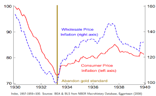
Margaret Jacobson presented her work with Eric Leeper and Bruce Preston on the end of the gold standard in the US in the 1930s. (Eric modestly stated his contribution to the paper as finding the matlab color code for gold, as shown in the graph.)  Margaret and Eric interpret the fiscal statements of the Roosevelt Administration to say that they would run unbacked deficits until the price level returned to its previous level, the \(P^\ast\) in my above equation.  Much discussion followed on how governments today, if they really want inflation, could achieve something similar.

 Part II Monetary Policy 

Chris Sims took on that issue directly. If you want inflation, just running big deficits might not help. Hundreds of years in which governments built up hard-won reputations that when they borrow money, they pay it off, are hard to upend immediately. Even if you want to break that expectation -- all our governments have mixed promises of stimulus now with deficit reduction later.  A devaluation would help, but we don't have a gold standard against which to devalue, and not everyone can devalue relative to each other's currency.

Chris' bottom line is a lot like Margaret and Eric's, and my fiscal Taylor rule,

Coordinating fiscal and monetary policy so that both are explicitly contingent on reaching an inflation target — not only interest rates low, but no tax increases or spending cuts until inflation rises. 

But,

• This might work because it would represent such a shift in political economy that people would rethink their inflation expectations.

Chris led a long discussion including thoughts on rational expectations -- it's a stretch to impose rational expectations on policies that have never been tried before (though our history lesson reminded us just how few genuinely novel policies there are!)

Steve Williamson followed with a thoughtful model full of surprising results. The stock of money does not matter, but fed transfers to the treasury do. (I hope I got that right!)

My presentation (slides also  here  on my webpage) took on the "agenda" question. The basic fiscal equation is
\[\frac{B_{t-1}}{P_t} = E_t \sum M_{t,t+j} s_{t+j} \]
For the project of matching history, data, analyzing policy and finding better regimes, I opined we have spent too much time on the \(s\) fiscal part, and not nearly enough time on the \(M\) discount rate part, or the \(B\) part, which I map to monetary policy.

I argued that in order to understand the cyclical variation of inflation -- in recessions inflation declines while \(B\) is rising and \(s\) is declining -- we need to focus on discount rate variation. More generally, changes in the value of government debt due to interest rate variation are plausibly much bigger than changes in expected surpluses. As interest rates rise, government debt will be worth a lot less, an additionan inflationary pressure that is often overlooked.

Then I presented short versions of recent papers analyzing monetary policy in the fiscal theory of the price level. Interest rate targets with no change in surpluses can determine expected inflation, but the neo-Fisherian conundrum remains.

Harald Uhlig presented a skeptical view, provoking much discussion.  Some main points: large debt and deficits are not associated with inflation, and M2 demand is stable.

I found Harald's critique quite useful. Even if you don't agree with something, knowing that this is how a really sharp and well informed macroeconomist perceives the issues is a vital lesson. I answered somewhat impertinently that we addressed these issues 15 years ago: High debt comes with large expected surpluses, just as in financing a war, because governments want to borrow without creating inflation. The stability of M2 velocity does not isolate cause and effect. The chocolate/GDP ratio is stable too, but eating more chocolate will not increase GDP.

But Harald knows this, and his overall point resonates: You guys need to find something like MV=PY that easily organizes historical events. The obvious graph doesn't work. Irving Fisher came up with MV=PY, but it took Friedman and Schwartz using it to make the idea come alive. That is the purpose of the whole conference.

Francesco Bianchi presented his work with Leonardo Melosi on the Great Recession. New Keynesian models typically predict huge deflation at the zero bound. Why didn't this happen? They specify a model with shifting fiscal vs money dominant regimes. The standard model specifies that once we leave the zero bound we go right back to a money-dominant, Taylor-rule regime with passive fiscal policy. However, if there is a chance of going back to a fiscal-dominant regime for a while, that changes expectations of inflation at the end of the zero bound. Even small changes in those expectations have big effects on inflation during the zero bound (Shameless plug for the New Keynesian Liquidity Trap which explains this point very simply.) So, as you see in the graph above, the "benchmark" model which includes a probability of reverting to a fiscal regime after the zero bound, produces the mild recession and disinflation we have seen, compared to the standard model prediction of a huge depression.

Fiscal policy is political of course. Campbell Leith presented, among other things,  an intriguing tour of how political scientists think about political determinants of debt and deficits. My snarky quip, we learned with great precision that political scientists don't know a heck of a lot more than we do! But if so, that is also wisdom.

Part III International

red line regime switching probability of 30%, blue line 0 % 

Alexander Kriwoluzky presented thoughts on a fiscal theory of exchange rates, applying it to the US vs. Germany, the abandonment of the gold standard and switch to floating rates in the early 1970s. An exchange rate peg means that Germany must import US fiscal policy as well, importing the deficits that support more inflation. Germany didn't want to do that.  People knew that, so a shift to floating rates was in the air. Expectations of that shift can explain the interest differential and apparent failure of uncovered interest parity.

Last but certainly not least, Bartosz Maćkowiak presented a thoughtful analysis of "Monetary-Fiscal Interactions and the Euro Area’s Malaise" joint work with Marek Jarosińsky.

Echoing the fiscal Taylor rule idea running through so many talks, they propose a fiscal rule
\[ S_{n,t} = \Psi_n + \Psi_B \left( B_{n,t-1} - \sum_n \theta_n B_{n,t-1} \right) + \psi_n (Y_{n,t}-Y_n) \]
In words, each country's surplus must react to that country's debt \(B_n\), but total EU surpluses do not react to total EU debt. In this way, the EU is "Ricardian" or "fiscal passive" for each country, but it is "non-Ricardian" or "fiscal active" for the EU as a whole. In their simulations, this fiscal commitment has the same beneficial effects running through Leeper and Jabcobson, Bianchi and Melosi, Sims, and others -- but maintaining the idea that individual countries pay their debts.

A big thanks to the Harris School and the Becker-Friedman Institute who sponsored the conference.

Neo-Fisherian caveats

Raise interest rates to raise inflation? Lower interest rates to lower inflation? It's not that simple.

A correspondent from an emerging market wrote enthusiastically. His country has somewhat too high inflation, currency depreciation and slightly negative real rates. A discussion is going on about raising rates to combat inflation. Do I think that lowering rates in this circumstance is instead the way to go about it?

As you can tell, posing the question this way makes me very uncomfortable! So, thinking out loud, why might one pause at jumping this far, this fast?

Fiscal policy.  Fiscal policy deeply underlies monetary policy. In my own "Fisherian" explorations, the fiscal theory of price level is a deep foundation. If the government is printing up money to pay its bills, the central bank can do what it wants with interest rates, inflation is coming anyway.


Conversely, underlying the decline in inflation in the US, Europe, and Japan is an extraordinary demand for nominal government debt.

Bond markets seem to think we'll pay it off. And that is not too terribly an irrational expectation. Sovereign debts are self-inflicted wounds. A little structural reform to get growing again, tweaks to social security and medicare, and next thing you know we're back in the 1990s and wondering what to do when all the government bonds are paid off. Also, valuation is more about discount rates than cashflows. People seem happy -- for now -- to hold government debt despite unusually low prospective returns.

My correspondent answers that his country is actually doing well fiscally.  However, his country is also a bit low on reserves and having exchange rate and capital flight problems.

But current deficits are not that important to inflation either in theory or in fact. The fiscal policy that matters is expectations of very long term stability, not just a few years of surpluses. Also, contingent liabilities matter a lot. If investors in government debt see a government that will bail out all and sundry in the next downturn, or faces political risks, even temporary surpluses are not an assurance to investors.  (Craig Burnside, Marty Eichenbaum and Sergio Rebelo's "Prospective Deficits and the Asian Currency Crises, in the JPE and ungated here is a brilliant paper on this point.)

Rational expectations. The Fisherian proposition also relies deeply on rational expectations. In the simplest version, \( i_t = r + E_t \pi_{t+1} \), people see nominal interest rates rise, they expect inflation to be higher, so they raise their prices. As a result of that expectation inflation is, on average, higher. (Loose story alert.)

How do they expect such a thing? Well,  rational expectations is sensible when there is a long history in one regime. People see higher interest rates, they remember times of high interest rates in the past, like the late 1970s, so they ratchet up their inflation expectations. Or, people see higher interest rates, and they've gotten used to the Fed raising interest rates when the Fed sees inflation coming, so they raise their expectations. The motto of rational expectations is "you can't fool all of the people all of the time," not "you can never fool anyone," nor "people are clairvoyant."

The Fisherian prediction relies on the interest rate change to be credible, long-lasting, and to lead to the right expectations. A one-off experiment, that might be read as cover for a dovish desire to boost growth at the expense of more inflation, and that might be quickly reversed doesn't really map to the equations. Europe and Japan, stuck at the zero bound, with a fiscal bonanza (low interest costs on the debt) and slowly decreasing inflation expectations is much more consistent with those equations.

Liquidity. When interest rates are positive and money does not pay interest, lowering rates means more money in the system, and potentially more lending too. This classic liquidity channel, which goes the other way, is absent for the US, UK, Japan and Europe, since we're at the zero bound and since reserves pay interest.  (Granted, I couldn't get the equations of the liquidity effect to be large enough to offset the Fisher effect, but that depends on the particulars of a model. )

Successful disinflations. Disinflations are a combination of fiscal policy, monetary policy, expectations, and liquidity. Tom Sargent's classic ends of four hyperinflations tells the story beautifully.

Large inflations result from intractable fiscal problems, not central bank stupidity. In Tom's examples, the government solves the fiscal problem; not just immediately, but credibly solves it for the forseeable future. For example, the German government in the 1920s faced enormous reparations payments. Renegotiating these payments fixed the underlying fiscal problem. When the long-term fiscal problem was fixed, inflation stopped immediately. Since everybody knew what the fiscal problem was, expectations were quickly rational.

The end of inflation coincided with a large money expansion and a steep reduction in nominal interest rates. During a time of high inflation, people use as little money as possible. With inflation over, real money demand expands.  There was no period of monetary stringency or interest-rate raising preceding these disinflations.

So these are great examples in which the Fisher story works well -- lower interest rates correspond to lower inflation, immediately. But you can see that lower interest rates are not the whole story. The central bank of Germany 1922 could not have stopped inflation on its own by lowering rates.  I suspect the same is true of high inflation countries today -- usually something is wrong other than just the history of interest rates.

So, apply new theories with caution!

To the raising interest rates question for the US and Europe, some of the same considerations apply. We won't have any liquidity effects, as central banks are planning to just pay more interest on abundant reserves. Higher real interest rates will raise fiscal interest costs, which is an inflationary shock by fiscal theory considerations. The big question is expectations. Will people read higher interest rates as a warning of inflation about to break out, or as a sign that inflation will be even lower?

The Habit Habit

The Habit Habit. This is an essay expanding slightly on a talk I gave at the University of Melbourne's excellent "Finance Down Under" conference. The slides

(Note: This post uses mathjax for equations and has embedded graphs. Some places that pick up the post don't show these elements. If you can't see them or links come back to the original. Two shift-refreshes seem to cure Safari showing "math processing error".)

Habit past: I start with a quick review of the habit model. I highlight some successes as well as areas where the model needs improvement, that I think would be productive to address.

Habit present: I survey of many current parallel approaches including long run risks, idiosyncratic risks, heterogenous preferences, rare disasters, probability mistakes -- both behavioral and from ambiguity aversion -- and debt or institutional finance. I stress how all these approaches produce quite similar results and mechanisms. They all introduce a business-cycle state variable into the discount factor, so they all give rise to more risk aversion in bad times. The habit model, though less popular than some alternatives, is at least still a contender, and more parsimonious in many ways,

Habits future: I speculate with some simple models that time-varying risk premiums as captured by the habit model can produce a theory of risk-averse recessions, produced by varying risk aversion and precautionary saving, as an alternative to  Keynesian flow constraints or new Keynesian intertemporal substitution. People stopped consuming and investing in 2008 because they were scared to death, not because they wanted less consumption today in return for more consumption tomorrow.

Throughout, the essay focuses on challenges for future research, in many cases that seem like low hanging fruit. PhD students seeking advice on thesis topics: I'll tell you to read this. It also may be useful to colleagues as a teaching note on macro-asset pricing models. (Note, the parallel sections of my coursera class "Asset Pricing" cover some of the same material.)

I'll tempt you with one little exercise taken from late in the essay.


A representative consumer with a fixed habit \(x\) lives in a permanent income economy, with endowment \(e_0\) at time 0 and random endowment \(e_1\) at time 1. With a discount factor \(\beta=R^f=1\), the problem is

\[ \max\frac{(c_{0}-x)^{1-\gamma}}{1-\gamma}+E\left[ \frac {(c_{1}-x)^{1-\gamma}}{1-\gamma}\right] \] \[ c_{1} = e_{0}-c_{0} +e_{1} \] \[ e_{1} =\left\{ e_{h},e_{l}\right\} \; pr(e_{l})=\pi. \] The solution results from the first order condition \[ \left( c_{0}-x\right) ^{-\gamma}=E\left[ (c_{1}-x)^{-\gamma}\right] \] i.e., \[ \left( c_{0}-x\right) ^{-\gamma}=\pi(e_{0}-c_{0}+e_{l}-x)^{-\gamma}% +(1-\pi)(e_{0}-c_{0}+e_{h}-x)^{-\gamma}% \] I solve this equation numerically for \(c_{0}\).

The first picture shows consumption \(c_0\) as a function of first period endowment \(e_0\) for \(e_{h}=2\), \(e_{l}=0.9\), \(x=1\), \(\gamma=2\) and \(\pi=1/100\).

The case that one state is a rare disaster is not special. In a general case, the consumer starts to focus more and more on the worst-possible state as risk aversion rises. Therefore, the model with any other distribution and the same worst-possible state looks much like this one.

Watch the blue \(c_0\) line first. Starting from the right, when first-period endowment \(e_{0}\) is abundant, the consumer follows standard permanent income advice. The slope of the line connecting initial endowment \(e_{0}\) to consumption \(c_{0}\) is about 1/2, as the consumer splits his large endowment \(e_{0}\) between period 0 and the single additional period 1.

As endowment \(e_{0}\) declines, however, this behavior changes. For very low endowments \(e_{0}\approx 1\) relative to the nearly certain better future \(e_{h}=2\), the permanent income consumer would borrow to finance consumption in period 0. The habit consumer reduces consumption instead. As endowment \(e_{0}\) declines towards \(x=1\), the marginal propensity to consume becomes nearly one. The consumer reduces consumption one for one with income.

The next graph presents marginal utility times probability, \(u^{\prime}(c_{0})=(c_{0}-x)^{-\gamma}\), and \(\pi_{i}u^{\prime}(c_{i})=\pi _{i}(c_{i}-x)^{-\gamma},i=h,l\). By the first order condition, the former is equal to the sum of the latter two. \ But which state of the world is the more important consideration? When consumption is abundant in both periods on the right side of the graph, marginal utility \(u^{\prime}(c_{0})\) is almost entirely equated to marginal utility in the 99 times more likely good state \((1-\pi)u^{\prime}(c_{h})\). So, the consumer basically ignores the bad state and acts like a perfect foresight or permanent-income intertemporal-substitution consumer, considering consumption today vs. consumption in the good state.

In bad times, however, on the left side of the graph, if the consumer thinks about leaving very little for the future, or even borrowing, consumption in the unlikely bad state approaches the habit. Now the marginal utility of the bad state starts to skyrocket compared to that of the good state. The consumer must leave some positive amount saved so that the bad state does not turn disastrous -- even though he has a 99% chance of doubling his income in the next period (\(e_{h}=2\), \(e_{0}=1\)). Marginal utility at time 0, \(u^{\prime }(c_{0})\) now tracks \(\pi_{l}u^{\prime}(c_{l})\) almost perfectly.

In these graphs, then, we see behavior that motivates and is captured by many different kinds of models:

1. Consumption moves more with income in bad times.

This behavior is familiar from buffer-stock models, in which agents wish to smooth intertemporally, but can't borrow when wealth is low....

2. In bad times, consumers start to pay inordinate attention to rare bad states of nature.

This behavior is similar to time-varying rare disaster probability models, behavioral models, or to minimax ambiguity aversion models. At low values of consumption, the consumer's entire behavior \(c_{0}\) is driven by the tradeoff between consumption today \(c_{0}\) and consumption in a state \(c_{l}\) that has a 1/100 probability of occurrence, ignoring the state with 99/100 probability.

This little habit model also gives a natural account of endogenous time-varying attention to rare events.

The point is not to argue that habit models persuasively dominate the others. The point is just that there seems to be a range of behavior that theorists intuit, and that many models capture.

When consumption falls close to habit, risk aversion rises, stock prices fall, so by Q theory investment falls. We nearly have a multiplier-accelerator, due to rising risk aversion in bad times: Consumption falls with mpc approaching one, and investment falls as well. The paper gives some hints about how that might work in a real model.

Deflation Puzzle

Larry Summers writes an eloquent FT column "A world stumped by stubbornly low inflation"

Market measures of inflation expectations have been collapsing and on the Fed’s preferred inflation measure are now in the range of 1-1.25 per cent over the next decade.

Inflation expectations are even lower in Europe and Japan. Survey measures have shown sharp declines in recent months. Commodity prices are at multi-decade lows and the dollar has only risen as rapidly as in the past 18 months twice during the past 40 years when it has fluctuated widely

And the Fed is forecasting a return to its 2 per cent inflation target on the basis of models that are not convincing to most outside observers. 

Central bankers [at the G20 meeting] communicated a sense that there was relatively little left that they can do to strengthen growth or even to raise inflation. This message was reinforced by the highly negative market reaction to Japan’s move to negative interest rates.

So why is inflation slowly declining despite our central banks' best efforts? Here is a stab at an answer. I emphasize the central logical points with bullets.

• Interest rates have two effects on inflation: a short-run "liquidity" effect, and a long-run "expected inflation" or "Fisher" effect.  

In normal times, to raise interest rates, the central bank sells bonds, which soaks up money. Less money drives up interest rates as people bid to borrow a smaller supply, and less money also reduces "demand," which reduces inflation.  In the long run, higher inflation and higher interest rates go together, as they did in the 1980s.

However, we are now in a classic "liquidity trap." Interest rates have been zero since 2008. Money and bonds are perfect substitutes. The proof of that is in the pudding: the Fed massively increased excess reserves from less than $50 billion to almost $3,000 billion, and inflation keeps trundling down.

• In a liquidity trap, the liquidity effect is absent. 

The liquidity effect will remain absent as the Fed starts raising interest rates, and would remain absent if the Fed were to cut rates or reduce them below zero as other central banks are doing. You can't have more than perfect liquidity.

The Fed isn't even planning to try. It plans to keep the $3,000 billion of excess reserves outstanding and raise interest rates by raising the interest rate on reserves. There will be no open market operations, no "tightening" associated with this interest rate raise.  But even if it did, we're $2,950 billion of excess reserves away from any liquidity effect, so it wouldn't matter.

• When the liquidity effect is absent, the expected inflation effect is all that remains. Inflation must follow interest rates. 

Central banks thought they were raising inflation by lowering interest rates, following experience from the normal-times liquidity-effect correlation between lower interest rates and higher inflation. But that experience does not apply when its liquidity effect is turned off.

With no liquidity effect, lowering interest rates further below zero can only, slowly, lower inflation further. Central banks desiring inflation may have followed a classic pedal mis-application.

Do I "believe" this story? Belief has no place in science. It is the simplest coherent story that explains the last few years, not needing lots of frictions, irrationalities, and other assumptions. I have some equations to back it up. But we don't "believe" anything at least until it's published and has survived critical examination, replication and dissection. Still, I think it merits consideration.

Shh. I like zero inflation. If central banks have the wrong pedal but are driving the right speed anyway, why wake them up? Even Larry seems to have given up on the Phillips curve:

...suppose that officials were comfortable with current policy settings based on the argument that Phillips curve models predicted that inflation would revert over time to target due to the supposed relationship between unemployment and price increases.

There is no sign of the dreaded "deflation vortex," any more than there is any sign of dreaded monetary hyperinflation. We're drifting down to the Friedman rule. As Larry emphasizes, don't get excited over forecasts from models that rather spectacularly did not forecast where we are today. 
Central banks' desire for 2% inflation, and the Fed's rather puzzling interpretation of its "price stability" mandate to mean perpetual 2% inflation may also be relics of the bygone liquidity-effect regime. 

Appreciate the first half of the column which turns the signs around. It's a great bit of rhetoric.

I have to register mild disagreement with Larry's "solution" to the supposed "problem," 

In all likelihood the important elements will be a combination of fiscal expansion drawing on the opportunity created by super low rates and, in extremis, further experimentation with unconventional monetary policies.

He doesn't say which monetary policies would work, given they have not done so yet. But these are topics for another day.

(Note: If quote and bullet formatting doesn't show up, come back to the original.)

Sanders multiplier magic

The critiques of Gerald Friedman's analysis of the Sanders economic plan  continue. The latest and most detailed and careful so far is by David and Christina Romer.

Bottom line:

1. The central idea in Friedman's analysis is that taking $1 from Peter to give to Paul raises overall income by 55 cents.  From this, you get multipliers from raising taxes and spending, from higher minimum wages, more unions, and so forth. 
2. I chuckle a little bit that so many economists who previously liked multipliers now don't like their logical conclusions. 
3. The Romers charge a serious, elementary arithmetic mistake in treating levels vs. growth rates. If they're right Friedman's whole analysis is just wrong on arithmetic.

The analysis

One might have expected that a sympathetic analysis of the Sanders plan would say, look, this is going to cost us a bit of growth, but the fairness and (claimed) better treatment of disadvantaged people are worth it.

Friedman's having none of that. In his analysis, the Sanders plan will also unleash a burst of growth, claims for which would make a fervent supply-sider like Art Laffer blush.

"The Sanders program... will raise the gross domestic product by 37% and per capita income by 33% in 2026; the growth rate of per capita GDP will increase from 1.7% a year to 4.5% a year." And, apparently, raise the growth rate permanently.

More stunning still are Friedman's claims about employment, shown at left here

and here.

Multipliers

So, where does this spurt of growth come from? The answer is the magic of multipliers.

But it's not just run of the mill fiscal stimulus multipliers.  After all, Friedman also says that the Sanders program would reduce the deficit, and by 2025 turn the Federal Budget to surplus!

How are multipliers so strong?

There seem to be two basic answers. First, Sanders assumes that there is a large multiplier from income transfers.

If the government takes $1 from rich Peter, and gives that $1 to poor Paul, overall income rises 55 cents! The one quote that makes this clearest is

The stimulus from regulator[y] changes is in Table 9. In general, the assumption is that wages have a multiplier of 0.9 compared with a multiplier of 0.35 for profits accruing to high-income persons. A wage increase coming out of profits, therefore, has a multiplier of 0.55.

It's also visible here explaining how a balanced budget still has a multiplier

the average value of the (governent spending) multiplier from 2017-26 is 0.89, falling from 1.25 to 0.87 as the output gap closes 

Other taxes are assumed to reduce effective demand with a multiplier of 0.35

[The] balance of revenue and spending programs will increase employment and economic growth because the spending program has a larger fiscal multiplier than do progressive tax increases. 

So tax $1 and spend $1 raises GDP by 54 cents.

He cites many standard sources for multipliers. He does not give a theory.  The standard story is that poor Paul consumes a lot more of his income, while rich Peter was investing it all in venture capital startups.  Consumption is good, savings is bad, so GDP rises.

From this central assumption, the rest of the magic follows.  Friedman creatively goes far beyond conventional deficit multipliers, to conjure multipliers out of tax increases, raises in the minimum wage, greater unionization, increased social program spending, and so forth. For example

 I assume that the Paycheck Fairness Act will raise women’s wages by 1% relative to men’s, and there will be an increase of 0.2% a year for the next decade.  I assume that 50% of the increased cost goes to higher prices and 50% comes from profits, and these are assumed to lower spending by higher income people with a multiplier of 0.35.

This, I think, is the central case. Admire it for its courage, and creative use of Keynesian arguments. These are the kind of interventions that most economists admit reduce growth, but some argue for on other grounds. But in Keynesian economics, taking money from low marginal propensity to consume people, and giving it to high marginal propensity to consume people raises GDP.

Snark

At this point, I stop in a bit of amusement at all the criticism. After all, these are just standard Keynesian arguments. The individual multipliers in Friedman's analysis are all conservative, and cite standard middle-of-the-road sources. The economists now so critical of this analysis, including the Romers, former democratic administration CEA chairs who wrote the open letter from past CEA chairs, and Paul Krugman, have been making big multiplier arguments for years to argue for more spending.  The "new Keynesian" academic literature includes multipliers far above two, so one can point to "science" if you wish. (Gauti Eggertsson, Christiano, Eichenbaum and Rebelo ; a simple example with multipliers as large as you want.)

The Romers are right to emphasize that multipliers only operate where "demand" is slack, and monetary policy doesn't steal the show. But the asterisks about fixed interest rates and output below "capacity" have been overlooked by the mainstream many times before. It's a rare Keynesian economist who ever thinks the economy is operating at full capacity. And Friedman has the former monetary asterisk, and he addresses the latter by claiming a large return to the labor force and increased productivity.

Even that view is not so out of the mainstream. For example,  Brad DeLong and Larry Summers wrote an influential Brookings paper arguing for very large fiscal multipliers, with some of the same flavor. There is hysterisis; a multiplier will bring people back to the labor market (as Friedman claims), those people will regain skills, productivity will increase; higher investment will give us better capital and also increase productivity. Demand creates its own supply.

Friedman is apparently just taking the consumption-first, poor-people-spend-more-than-rich-people, undergraduate ISLM analysis, with a bit of Delong-Summers hysterisis, to its logical conclusion. I agree in a way: take those ideas to their logical conclusion and you get silly propositions (old essay on that). Robbing Peter to pay Paul raises income; wasted government spending is good; theft improves the economy, transfers even from thrifty poor to spendthrift rich improve the economy, hurricanes are good for us, social programs, unions, minimum wages raise GDP, and so forth. Well, if the logical conclusions are patently silly, maybe one shouldn't have been making small versions of those arguments all along. Economic Homeopathy is not wisdom. 

Arithmetic 

But the Romers uncover a deeper puzzle. Even with these assumptions -- government spending multipliers around 0.8, and a transfer multiplier of around 0.55 -- you still don't get the wild increase in growth that Friedman claims. So how does he do it? Their answer: 

We have a conjecture about how Friedman may have incorrectly found such large effects. Suppose one is considering a permanent increase in government spending of 1% of GDP, and suppose one assumes that government spending raises output one-for-one. Then one might be tempted to think that the program would raise output growth each year by a percentage point, and so raise the level of output after a decade by about 10%. In fact, however, in this scenario there is no additional stimulus after the first year. As a result, each year the spending would raise the level of output by 1% relative to what it would have been otherwise, and so the impact on the level of output after a decade would be only 1%.

If this is right, it's absolutely damning. This is a question of arithmetic, not economics. (And I would have to swallow some of my above snark!) 

A clearer (maybe) example: The government spends an extra $1 for one year.  With a 1.0 multiplier GDP goes up $1 that year, period. If the government stops spending next year, GDP goes back to where it was. That's the conventional definition of multiplier, and the one that all Fridman's cited sources have in mind. Per Romers, Friedman misread that calculation and assumed the first $1 of spending raises GDP by $1 forever. In 10 years, you have a multiplier of 10! 

The Romers are cautious, and don't directly make this charge. It's not my job to get into the Hilary vs. Bernie whose-numbers-add-up fight. (At least someone here actually seems to care about numbers and economic plans!) But whether the spreadsheets make this arithmetic mistake or not is an answerable question. I hope to inspire someone with a spreadsheet and a nose for such things to check. This is a great time for a replication exercise! 

(Note: This post has pictures and quotes, which don't translate well when the post is picked up elswhere. If you're not seeing them, come back to the original.)

Update: Joakim Book tries to reproduce the numbers and comes up way short.

Update 2: Justin Wolfers at the New York Times did some old-fashioned journalism: He called up Friedman for a reaction.  The article is great, and clear. Yes, Friedman did the calculation as the Romers allege: An extra dollar of government spending today raises GDP permanently; an extra dollar of permanent government spending raises GDP growth permanently. That is at least not what the cited sources have in mind.

Negative rates and FTPL

I've devoted most of my monetary economics research agenda to the Fiscal Theory of the Price Level in the last two decades (collection here). This theory says, fundamentally, that money has value because the government accepts it for taxes, and inflation is fundamentally a fiscal phenomenon over which central banks' conventional tools -- open market operations trading money for government bonds -- have limited power.

Since I grew up in the 1970s, I figured the FTPL would have its day when inflation unexpectedly broke out, again, and central banks were powerless to stop it. I figured that the spread of interest-paying electronic money would so clearly undermine the foundations of MV=PY that its pleasant stories would be quickly abandoned as no longer relevant.

I may have been  exactly wrong on both points: It seems that uncontrolled disinflation or deflation will be the spark for adoption of FTPL ideas; that the equivalence of money and bonds at zero interest rates,  and central banks powerless to create inflation will be the trigger.

These thoughts are prodded by two pieces in the Economist, "Out of Ammo:" and "Unfamiliar Ways Forward" (HT and interesting discussion by Miles Kimball)

If you want inflation (a big if -- I don't, but let's go with the if) how do you get it? Ultra-low rates, huge bond purchases, and lots of talk (forward guidance, higher inflation targets) seem to have no effect. What can governments actually do?


"Out of ammo" explains

... At least some of them [politicians] have failed to grasp the need to have fiscal and monetary policy operating in concert....

... One such option is to finance public spending (or tax cuts) directly by printing money—known as a “helicopter drop”. Unlike QE, a helicopter drop bypasses banks and financial markets, and puts freshly printed cash straight into people’s pockets. The sheer recklessness of this would, in theory, encourage people to spend the windfall, not save it. 

The "recklessness" part is crucial. "Unfamiliar ways" has a more intricate scheme to communicate that recklessness

..a central bank and its finance ministry ... collude in printing money to pay for public spending (or tax cuts). ...the government announces a tax rebate and issues bonds to finance it, but instead of selling them to private investors swaps them for a deposit with the central bank. The central bank proceeds to cancel the bonds, and the government withdraws the money it has on deposit and gives it to citizens. “Helicopter money” of this sort—named in honour of a parable told by Milton Friedman, a famous economist—is as close as you can get to raining cash from a clear blue sky like manna from heaven, untouched by banks and financial markets.

Such largesse is, in effect, fiscal policy financed by money instead of bonds... But the unaccustomed drama—indeed, the apparent recklessness—of helicopter money could increase the expected inflation rate, encouraging taxpayers to spend rather than save.

Simpler, in my mind, the Treasury borrows and sends checks to voters. The Fed buys the bonds and then cancels them.

In addition to rather convoluted scheme, the pieces are not quite clear why the fiscal counterpart is necessary -- or why money has to be involved with fiscal policy.  That was not a central part of Friedman's helicopters. Miles is clearer about this:

the government give[s] away so much money that people would be convinced there was no way the government could ever sell enough bonds to soak that money up. 

This is clear and good FTPL thinking. The value of money is set by how much there is vs how much people expect the government to soak up via taxes -- or bond sales, backed by credible promises of future taxes.

If the government drops $100 in every voter's pocket but simultaneously announces "austerity" that taxes are going up $100 tomorrow, even helicopter drops would have no effect.

Helicopter drops are a clever fiscal signaling device. Canceling the bonds in the Economists plan is the crucial signaling device. They say "we are really going to be reckless."  When governments sell a lot of bonds, people think  the government is sooner or later going to soak up these bonds with taxes, and do not spend. That's the whole point -- bond sales are set up to raise revenue, not to create inflation.  The whole canceling the bonds thing in the Economists's plan, or the helicopter drama in Friedman's, is a clever psychological device, to convince people that no, the government is not going to raise taxes to soak money or underlying bonds up, so you'd better spend it now before it loses value.

Well if (if) our central banks want inflation, why not get out the helicopters?

Such shenanigans are not possible in the euro zone, where the ECB is forbidden by treaty from buying government bonds directly. Elsewhere they might work as follows: 

monetary financing is prohibited by the treaties underpinning the euro, for example

The US Federal reserve is similarly constrained to always buy something in return for creating money -- it can't send checks to voters.

Why?  The people who set up our monetary systems understood all this very well. Their memories were full of disastrous inflations, and they understood that printing money without clear promises that taxes would eventually soak up that money would lead quickly to inflation. So, yes, central banks are prohibited from doing the one thing that would most quickly produce inflation! For about the same reason that wise parents don't keep the car keys in the liquor cabinet.  (There are also all sorts of good political economy reasons that an independent central bank should not lend to specific businesses or send checks to voters.)

The Economist articles are also quite good at the evidence that current monetary policy is essentially powerless.

If policymakers appear defenceless in the face of a fresh threat to the world economy, it is in part because they have so little to show for their past efforts. The balance-sheets of the rich world’s main central banks have been pumped up to between 20% and 25% of GDP by the successive bouts of QE with which they have injected money into their economies (see chart 1). The Bank of Japan’s assets are a whopping 77% of GDP. Yet inflation has been persistently below the 2% goal that central banks aim for.

The power of open market operations -- buying bonds in return for money - is just dramatically refuted, at least at zero interest rates, by recent experience.

One way to get them back up might be to set a higher inflation target. But when inflation sits so persistently below today’s targets, persuading people that higher targets would produce higher rates will require action, not just words.

Or as I call it, the speak loudly because you have no stick policy. If central banks announce a 5% inflation target, and inflation goes down anyway, now what? Announce a 10% target?

Miles goes on about the power of negative interest rates to stoke inflation, which will be a topic for another day. If negative 2% real rates (2% inflation, 0% interest) didn't stoke "demand" and revive the extinct Phillips curve,  I don't see how negative 3% (2% inflation  -1% interest rate) or negative 5% will finally do the trick. In the standard models I've been playing with,  raising nominal interest rates, and committing to keep them there, is the way for central banks to raise expected inflation. That action would, however, also cool the economy, producing stagflation, and thus be particularly pointless.

I also fully admit that I'm cherry-picking the things I like from the Economist article, and ignoring all sorts of things that seem pretty silly to me. The point: I'm glad to see fiscal-theory thinking making its way out of academic debate into real-world commentary, if only in the "radical ideas" section.  Now, on to the "conventional wisdom" section!